Simple analyses of conjoint (factorial) experiments and visualization of results.
cj(
  data,
  formula,
  id = ~0,
  weights = NULL,
  estimate = c("amce", "frequencies", "mm", "amce_differences", "mm_differences"),
  feature_order = NULL,
  feature_labels = NULL,
  level_order = c("ascending", "descending"),
  by = NULL,
  ...
)
Arguments
| data | A data frame containing variables specified in |
|---|---|
| formula | A formula specifying a model to be estimated. ; all levels across features should be unique. For |
| id | An RHS formula specifying a variable holding respondent identifiers, to be used for clustering standard errors. |
| weights | An (optional) RHS formula specifying a variable holding survey weights. |
| estimate | A character string specifying an estimate type. Current options are average marginal component effects (or AMCEs, “amce”, estimated via |
| feature_order | An (optional) character vector specifying the names of feature (RHS) variables in the order they should be encoded in the resulting data frame. |
| feature_labels | A named list of “fancy” feature labels to be used in output. By default, the function looks for a “label” attribute on each variable in |
| level_order | A character string specifying levels (within each feature) should be ordered increasing or decreasing in the final output. This is mostly only consequential for plotting via |
| by | A formula containing only RHS variables, specifying grouping factors over which to perform estimation. |
| ... | Additional arguments to |
Value
A data frame with special class to facilitate plotting (e.g., “cj_amce”, “cj_mm”, etc.)
Details
The main function cj is a convenience function wrapper around the underlying estimation functions that provide for average marginal component effects (AMCEs), by default, via the amce function, marginal means (MMs) via the mm function, and display frequencies via cj_freqs and cj_props. Additional estimands may be supported in the future through their own functions and through the cj interface. Plotting is provided via ggplot2 for all types of estimates.
The only additional functionality provided by cj over the underlying functions is the by argument, which will perform operations on subsets of data, returning a single data frame. This can be useful, for example, for evaluating profile spillover effects and subgroup results, or in any situation where one might be inclined to use a for loop or lapply, calling cj repeatedly on subgroups.
Note: Some features of cregg (namely, the amce_diffs) function, or estimate = "amce_diff" here) only work with full factorial conjoint experiments. Designs involving two-way constraints between features are supported simply by expressing interactions between constrained terms in formula (again, except for amce_diffs). Higher-order constraints may be supported in the future.
See also
Functions: amce, mm, cj_freqs, mm_diffs, plot.cj_amce, cj_tidy
Data: immigration, taxes
Examples
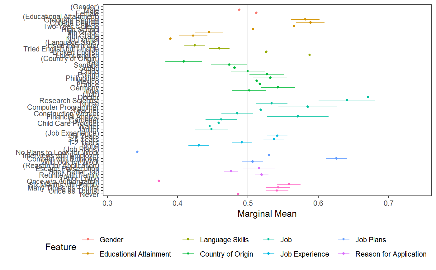
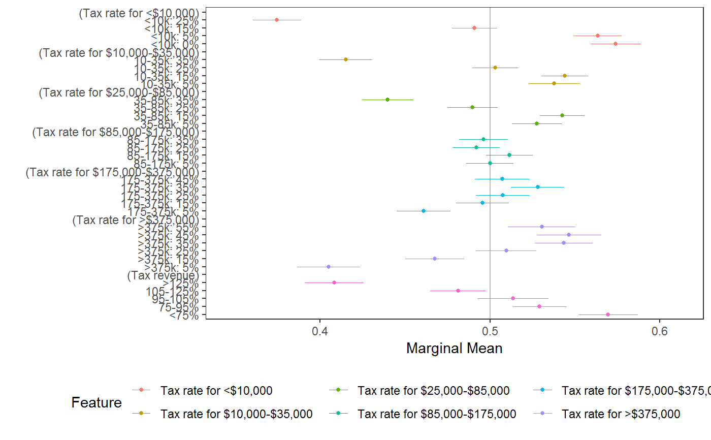
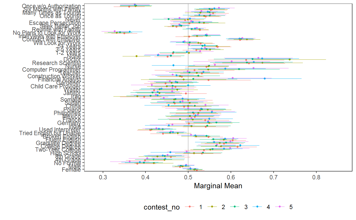
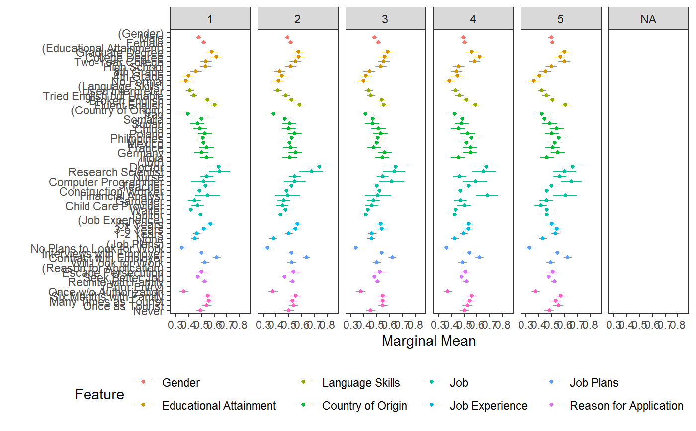
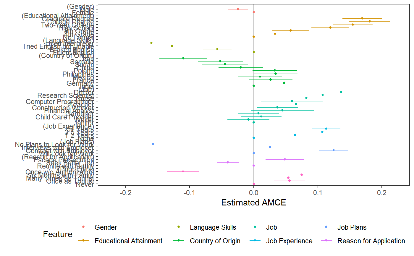
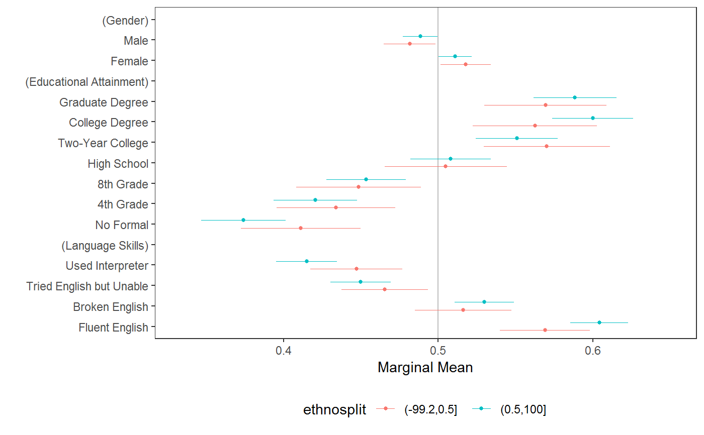
# \donttest{ # load data requireNamespace("ggplot2") data("immigration") immigration$contest_no <- factor(immigration$contest_no) data("taxes") # calculate MMs f1 <- ChosenImmigrant ~ Gender + Education + LanguageSkills + CountryOfOrigin + Job + JobExperience + JobPlans + ReasonForApplication + PriorEntry d1 <- cj(immigration, f1, id = ~ CaseID, estimate = "mm", h0 = 0.5) # plot MMs plot(d1, vline = 0.5)# calculate MMs for survey-weighted data d1 <- cj(taxes, chose_plan ~ taxrate1 + taxrate2 + taxrate3 + taxrate4 + taxrate5 + taxrate6 + taxrev, id = ~ ID, weights = ~ weight, estimate = "mm", h0 = 0.5) # plot MMs plot(d1, vline = 0.5)# MMs split by profile number stacked <- cj(immigration, f1, id = ~ CaseID, estimate = "mm", by = ~ contest_no) ## plot with grouping plot(stacked, group = "contest_no", vline = 0.5, feature_headers = FALSE)## subgroup analysis immigration$ethnosplit <- cut(immigration$ethnocentrism, 2) x <- cj(na.omit(immigration), ChosenImmigrant ~ Gender + Education + LanguageSkills, id = ~ CaseID, estimate = "mm", h0 = 0.5, by = ~ ethnosplit) plot(x, group = "ethnosplit", vline = 0.5)# combinations of/interactions between features immigration$language_entry <- interaction(immigration$LanguageSkills, immigration$PriorEntry, sep = "_") ## higher-order MMs for feature combinations cj(immigration, ChosenImmigrant ~ language_entry, id = ~CaseID, estimate = "mm", h0 = 0.5)#> outcome statistic feature #> 1 ChosenImmigrant mm language_entry #> 2 ChosenImmigrant mm language_entry #> 3 ChosenImmigrant mm language_entry #> 4 ChosenImmigrant mm language_entry #> 5 ChosenImmigrant mm language_entry #> 6 ChosenImmigrant mm language_entry #> 7 ChosenImmigrant mm language_entry #> 8 ChosenImmigrant mm language_entry #> 9 ChosenImmigrant mm language_entry #> 10 ChosenImmigrant mm language_entry #> 11 ChosenImmigrant mm language_entry #> 12 ChosenImmigrant mm language_entry #> 13 ChosenImmigrant mm language_entry #> 14 ChosenImmigrant mm language_entry #> 15 ChosenImmigrant mm language_entry #> 16 ChosenImmigrant mm language_entry #> 17 ChosenImmigrant mm language_entry #> 18 ChosenImmigrant mm language_entry #> 19 ChosenImmigrant mm language_entry #> 20 ChosenImmigrant mm language_entry #> level estimate std.error #> 1 Fluent English_Never 0.5963939 0.01794824 #> 2 Broken English_Never 0.5000000 0.01868574 #> 3 Tried English but Unable_Never 0.4211248 0.01813613 #> 4 Used Interpreter_Never 0.4209703 0.01908138 #> 5 Fluent English_Once as Tourist 0.6330409 0.01802151 #> 6 Broken English_Once as Tourist 0.5700000 0.01790043 #> 7 Tried English but Unable_Once as Tourist 0.5195936 0.01831354 #> 8 Used Interpreter_Once as Tourist 0.4458509 0.01830720 #> 9 Fluent English_Many Times as Tourist 0.6222222 0.01744591 #> 10 Broken English_Many Times as Tourist 0.5759768 0.01828850 #> 11 Tried English but Unable_Many Times as Tourist 0.5082956 0.01909682 #> 12 Used Interpreter_Many Times as Tourist 0.4579025 0.01945735 #> 13 Fluent English_Six Months with Family 0.6250000 0.01770276 #> 14 Broken English_Six Months with Family 0.6008902 0.01855907 #> 15 Tried English but Unable_Six Months with Family 0.5243902 0.01786358 #> 16 Used Interpreter_Six Months with Family 0.4843305 0.01840726 #> 17 Fluent English_Once w/o Authorization 0.4651163 0.01854707 #> 18 Broken English_Once w/o Authorization 0.3865906 0.01829631 #> 19 Tried English but Unable_Once w/o Authorization 0.3211144 0.01759690 #> 20 Used Interpreter_Once w/o Authorization 0.3151261 0.01724809 #> z p lower upper #> 1 5.370659e+00 7.844941e-08 0.5612160 0.6315718 #> 2 7.724017e-14 1.000000e+00 0.4633766 0.5366234 #> 3 -4.349064e+00 1.367201e-05 0.3855787 0.4566710 #> 4 -4.141720e+00 3.447109e-05 0.3835714 0.4583691 #> 5 7.382341e+00 1.555297e-13 0.5977194 0.6683624 #> 6 3.910520e+00 9.209754e-05 0.5349158 0.6050842 #> 7 1.069898e+00 2.846654e-01 0.4836997 0.5554875 #> 8 -2.957803e+00 3.098405e-03 0.4099695 0.4817324 #> 9 7.005779e+00 2.456151e-12 0.5880289 0.6564156 #> 10 4.154350e+00 3.262131e-05 0.5401320 0.6118217 #> 11 4.343984e-01 6.639992e-01 0.4708666 0.5457247 #> 12 -2.163577e+00 3.049681e-02 0.4197668 0.4960382 #> 13 7.061047e+00 1.652524e-12 0.5903032 0.6596968 #> 14 5.436168e+00 5.443869e-08 0.5645151 0.6372653 #> 15 1.365361e+00 1.721395e-01 0.4893783 0.5594022 #> 16 -8.512682e-01 3.946204e-01 0.4482529 0.5204081 #> 17 -1.880821e+00 5.999628e-02 0.4287647 0.5014679 #> 18 -6.198487e+00 5.700850e-10 0.3507305 0.4224507 #> 19 -1.016574e+01 2.819594e-24 0.2866251 0.3556037 #> 20 -1.071852e+01 8.332769e-27 0.2813204 0.3489317## constrained designs ## in a constrained design, some cells are unobserved: subset(cj_props(immigration, ~ Job + Education), Proportion == 0)#> Job Education Proportion #> 5 Financial Analyst No Formal 0 #> 8 Computer Programmer No Formal 0 #> 10 Research Scientist No Formal 0 #> 11 Doctor No Formal 0 #> 16 Financial Analyst 4th Grade 0 #> 19 Computer Programmer 4th Grade 0 #> 21 Research Scientist 4th Grade 0 #> 22 Doctor 4th Grade 0 #> 27 Financial Analyst 8th Grade 0 #> 30 Computer Programmer 8th Grade 0 #> 32 Research Scientist 8th Grade 0 #> 33 Doctor 8th Grade 0 #> 38 Financial Analyst High School 0 #> 41 Computer Programmer High School 0 #> 43 Research Scientist High School 0 #> 44 Doctor High School 0## MMs and AMCEs only use data from observed cells ## In `immigraation`, this means while the MM for `Job == "Janitor"` is an average ## across all levels of Education: mm(subset(immigration, Job == "Janitor"), ChosenImmigrant ~ Education)#> outcome statistic feature level estimate #> 1 ChosenImmigrant mm Educational Attainment No Formal 0.3344828 #> 2 ChosenImmigrant mm Educational Attainment 4th Grade 0.3962963 #> 3 ChosenImmigrant mm Educational Attainment 8th Grade 0.4782609 #> 4 ChosenImmigrant mm Educational Attainment High School 0.4791667 #> 5 ChosenImmigrant mm Educational Attainment Two-Year College 0.5439560 #> 6 ChosenImmigrant mm Educational Attainment College Degree 0.4578947 #> 7 ChosenImmigrant mm Educational Attainment Graduate Degree 0.5185185 #> std.error z p lower upper #> 1 0.02771408 12.06905 1.538950e-33 0.2801642 0.3888014 #> 2 0.02977646 13.30905 2.050813e-40 0.3379355 0.4546571 #> 3 0.02889725 16.55039 1.590622e-61 0.4216233 0.5348984 #> 4 0.03225671 14.85479 6.477049e-50 0.4159447 0.5423887 #> 5 0.03693028 14.72927 4.181974e-49 0.4715740 0.6163381 #> 6 0.03615604 12.66441 9.312345e-37 0.3870302 0.5287593 #> 7 0.03926878 13.20434 8.281792e-40 0.4415531 0.5954839## the MM for `Job == "Doctor"` is an average across only 3 levels of education: mm(subset(immigration, Job == "Doctor"), ChosenImmigrant ~ Education)#> outcome statistic feature level estimate #> 1 ChosenImmigrant mm Educational Attainment No Formal NA #> 2 ChosenImmigrant mm Educational Attainment 4th Grade NA #> 3 ChosenImmigrant mm Educational Attainment 8th Grade NA #> 4 ChosenImmigrant mm Educational Attainment High School NA #> 5 ChosenImmigrant mm Educational Attainment Two-Year College 0.6702703 #> 6 ChosenImmigrant mm Educational Attainment College Degree 0.7037037 #> 7 ChosenImmigrant mm Educational Attainment Graduate Degree 0.6453202 #> std.error z p lower upper #> 1 NA NA NA NA NA #> 2 NA NA NA NA NA #> 3 NA NA NA NA NA #> 4 NA NA NA NA NA #> 5 0.03459500 19.37477 1.260167e-83 0.6024653 0.7380752 #> 6 0.03590837 19.59721 1.633525e-85 0.6333246 0.7740828 #> 7 0.03360880 19.20093 3.635303e-82 0.5794482 0.7111922## Use `cj_props()` to see constraints: subset(cj_props(immigration, ~ Job + Education), Job == "Doctor" & Proportion != 0)#> Job Education Proportion #> 55 Doctor Two-Year College 0.01325215 #> 66 Doctor College Degree 0.01160458 #> 77 Doctor Graduate Degree 0.01454155## Substantively, the MM of "Doctor" might be higher than other levels of `Job` ## this could be due to the feature itself or due to the fact that it is constrained ## with a different subset of other feature levels than alternative levels of `Job` ## this may mean analysts want to report MMs (or AMCEs) only for the unconstrained levels: elev <- c("Two-Year College", "College Degree", "Graduate Degree") jlev <- c("Financial Analyst", "Computer Programmer", "Research Scientist", "Doctor") mm(subset(immigration, Education %in% elev), ChosenImmigrant ~ Job)#> outcome statistic feature level estimate std.error #> 1 ChosenImmigrant mm Job Janitor 0.5056180 0.02163756 #> 2 ChosenImmigrant mm Job Waiter 0.5215146 0.02072601 #> 3 ChosenImmigrant mm Job Child Care Provider 0.5432781 0.02137831 #> 4 ChosenImmigrant mm Job Gardener 0.5597826 0.02113051 #> 5 ChosenImmigrant mm Job Financial Analyst 0.5708419 0.02243047 #> 6 ChosenImmigrant mm Job Construction Worker 0.5369369 0.02116759 #> 7 ChosenImmigrant mm Job Teacher 0.6175943 0.02059314 #> 8 ChosenImmigrant mm Job Computer Programmer 0.5848708 0.02116695 #> 9 ChosenImmigrant mm Job Nurse 0.6128440 0.02086681 #> 10 ChosenImmigrant mm Job Research Scientist 0.6407407 0.02064831 #> 11 ChosenImmigrant mm Job Doctor 0.6709091 0.02003755 #> z p lower upper #> 1 23.36761 9.127274e-121 0.4632091 0.5480268 #> 2 25.16232 1.036043e-139 0.4808924 0.5621369 #> 3 25.41258 1.830936e-142 0.5013774 0.5851788 #> 4 26.49167 1.208924e-154 0.5183676 0.6011977 #> 5 25.44939 7.169262e-143 0.5268790 0.6148048 #> 6 25.36599 5.987418e-142 0.4954492 0.5784247 #> 7 29.99030 1.313363e-197 0.5772324 0.6579561 #> 8 27.63133 4.679276e-168 0.5433844 0.6263573 #> 9 29.36933 1.353960e-189 0.5719458 0.6537422 #> 10 31.03114 2.049693e-211 0.6002708 0.6812107 #> 11 33.48258 8.641056e-246 0.6316362 0.7101820#> outcome statistic feature level estimate #> 1 ChosenImmigrant mm Educational Attainment No Formal NA #> 2 ChosenImmigrant mm Educational Attainment 4th Grade NA #> 3 ChosenImmigrant mm Educational Attainment 8th Grade NA #> 4 ChosenImmigrant mm Educational Attainment High School NA #> 5 ChosenImmigrant mm Educational Attainment Two-Year College 0.6134094 #> 6 ChosenImmigrant mm Educational Attainment College Degree 0.6372981 #> 7 ChosenImmigrant mm Educational Attainment Graduate Degree 0.6051560 #> std.error z p lower upper #> 1 NA NA NA NA NA #> 2 NA NA NA NA NA #> 3 NA NA NA NA NA #> 4 NA NA NA NA NA #> 5 0.01839689 33.34311 9.168440e-244 0.5773522 0.6494667 #> 6 0.01842787 34.58338 4.491516e-262 0.6011801 0.6734161 #> 7 0.01801006 33.60100 1.622146e-247 0.5698570 0.6404551## or, present estimates excluding constrained levels: mm(subset(immigration, !Education %in% elev), ChosenImmigrant ~ Job)#> outcome statistic feature level estimate std.error #> 1 ChosenImmigrant mm Job Janitor 0.4203822 0.01489092 #> 2 ChosenImmigrant mm Job Waiter 0.4066608 0.01454294 #> 3 ChosenImmigrant mm Job Child Care Provider 0.4204452 0.01417421 #> 4 ChosenImmigrant mm Job Gardener 0.4127273 0.01484507 #> 5 ChosenImmigrant mm Job Financial Analyst NA NA #> 6 ChosenImmigrant mm Job Construction Worker 0.4587489 0.01500467 #> 7 ChosenImmigrant mm Job Teacher 0.4690813 0.01483345 #> 8 ChosenImmigrant mm Job Computer Programmer NA NA #> 9 ChosenImmigrant mm Job Nurse 0.4974705 0.01451942 #> 10 ChosenImmigrant mm Job Research Scientist NA NA #> 11 ChosenImmigrant mm Job Doctor NA NA #> z p lower upper #> 1 28.23078 2.450898e-175 0.3911965 0.4495678 #> 2 27.96277 4.610542e-172 0.3781572 0.4351645 #> 3 29.66269 2.326579e-193 0.3926642 0.4482261 #> 4 27.80230 4.068329e-170 0.3836315 0.4418231 #> 5 NA NA NA NA #> 6 30.57374 2.734786e-205 0.4293403 0.4881575 #> 7 31.62321 1.771151e-219 0.4400082 0.4981543 #> 8 NA NA NA NA #> 9 34.26242 2.849362e-257 0.4690129 0.5259280 #> 10 NA NA NA NA #> 11 NA NA NA NA#> outcome statistic feature level estimate #> 1 ChosenImmigrant mm Educational Attainment No Formal 0.3895112 #> 2 ChosenImmigrant mm Educational Attainment 4th Grade 0.4222002 #> 3 ChosenImmigrant mm Educational Attainment 8th Grade 0.4444444 #> 4 ChosenImmigrant mm Educational Attainment High School 0.5075226 #> 5 ChosenImmigrant mm Educational Attainment Two-Year College 0.5398773 #> 6 ChosenImmigrant mm Educational Attainment College Degree 0.5631825 #> 7 ChosenImmigrant mm Educational Attainment Graduate Degree 0.5675254 #> std.error z p lower upper #> 1 0.01100389 35.39758 1.860555e-274 0.3679440 0.4110784 #> 2 0.01099526 38.39837 0.000000e+00 0.4006499 0.4437505 #> 3 0.01111714 39.97831 0.000000e+00 0.4226552 0.4662336 #> 4 0.01119635 45.32927 0.000000e+00 0.4855781 0.5294670 #> 5 0.01380270 39.11390 0.000000e+00 0.5128245 0.5669301 #> 6 0.01385316 40.65372 0.000000e+00 0.5360308 0.5903342 #> 7 0.01384257 40.99855 0.000000e+00 0.5403944 0.5946563# }