Plot AMCE estimates, MM descriptives, and frequency plots

ggplot2-based plotting of conjoint AMCEs estimates and MMs, and differences

# S3 method for cj_amce
plot(
  x,
  group = attr(x, "by"),
  feature_headers = TRUE,
  header_fmt = "(%s)",
  size = 1,
  xlab = "Estimated AMCE",
  ylab = "",
  legend_title = if (is.null(group)) "Feature" else group,
  legend_pos = "bottom",
  xlim = NULL,
  vline = 0,
  vline_color = "gray",
  theme = ggplot2::theme_bw(),
  ...
)

# S3 method for cj_diffs
plot(
  x,
  group = attr(x, "by"),
  feature_headers = TRUE,
  header_fmt = "(%s)",
  size = 1,
  xlab = "Estimated Difference",
  ylab = "",
  legend_title = if (is.null(group)) "Feature" else group,
  legend_pos = "bottom",
  xlim = NULL,
  vline = 0,
  vline_color = "gray",
  theme = ggplot2::theme_bw(),
  ...
)

# S3 method for cj_freqs
plot(
  x,
  group = attr(x, "by"),
  feature_headers = TRUE,
  header_fmt = "(%s)",
  xlab = "",
  ylab = "Frequency",
  legend_title = if (is.null(group)) "Feature" else group,
  legend_pos = "bottom",
  theme = ggplot2::theme_bw(),
  ...
)

# S3 method for cj_mm
plot(
  x,
  group = attr(x, "by"),
  feature_headers = TRUE,
  header_fmt = "(%s)",
  size = 1,
  xlab = "Marginal Mean",
  ylab = "",
  legend_title = if (is.null(group)) "Feature" else group,
  legend_pos = "bottom",
  xlim = NULL,
  vline = 0,
  vline_color = "gray",
  theme = ggplot2::theme_bw(),
  ...
)

Arguments

x	A data frame returned from cj or mm.
group	Optionally a character string specifying a grouping factor. This is useful when, for example, subgroup analyses or comparing AMCEs for different outcomes. An alternative is to use facet_wrap for faceted graphics.
feature_headers	A logical indicating whether to include headers for each feature to visually separate levels for each feature (beyond the color palette).
header_fmt	A character string specifying a fmt argument to sprintf, which will be used when generating the feature headers (if feature_headers = TRUE).
size	A numeric value specifying point size in geom_point.
xlab	A label for the x-axis
ylab	A label for the y-axis
legend_title	A character string specifying a label for the legend.
legend_pos	An argument forwarded to the legend.position argument in theme.
xlim	A two-element number vector specifying limits for the x-axis. If NULL, a default value is calculated from the data.
vline	Optionally, a numeric value specifying an x-intercept for a vertical line. This can be useful in distinguishing the midpoint of the estimates (e.g., a zero line for AMCEs).
vline_color	A character string specifying a color for the vline.
theme	A ggplot2 theme object
...	Ignored.

Value

A ggplot2 object

Details

These are convenience functions for quickly plotting results from cregg. Because plot returns ggplot2 objects, these are easily manipulated using standard ggplot2 operations.

Note that ggplot2, by default, sorts factors (like feature names here) in what might be the opposite order of what you would expect and in the opposite order that cregg functions sort their output.

See also

amce, mm

Examples

# \donttest{
require("ggplot2")
#> Loading required package: ggplot2
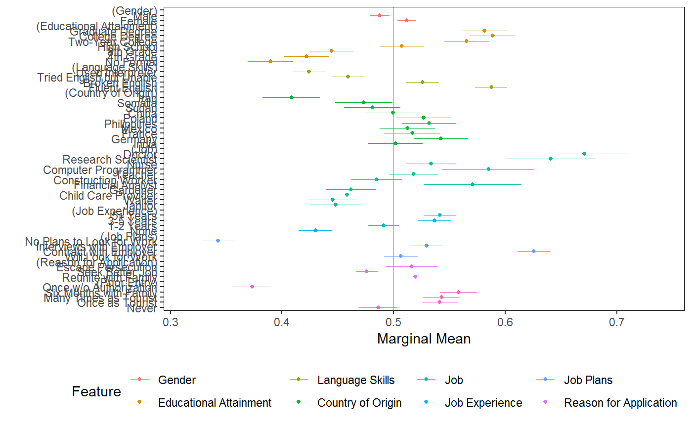
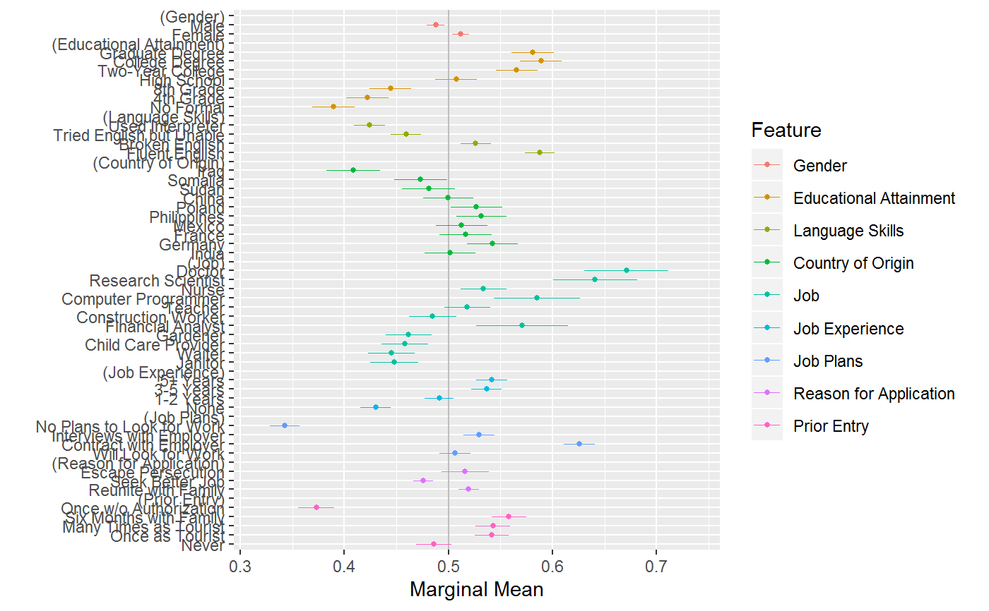
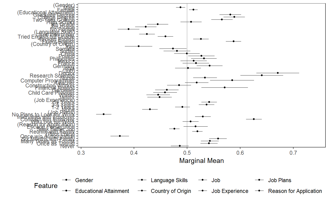
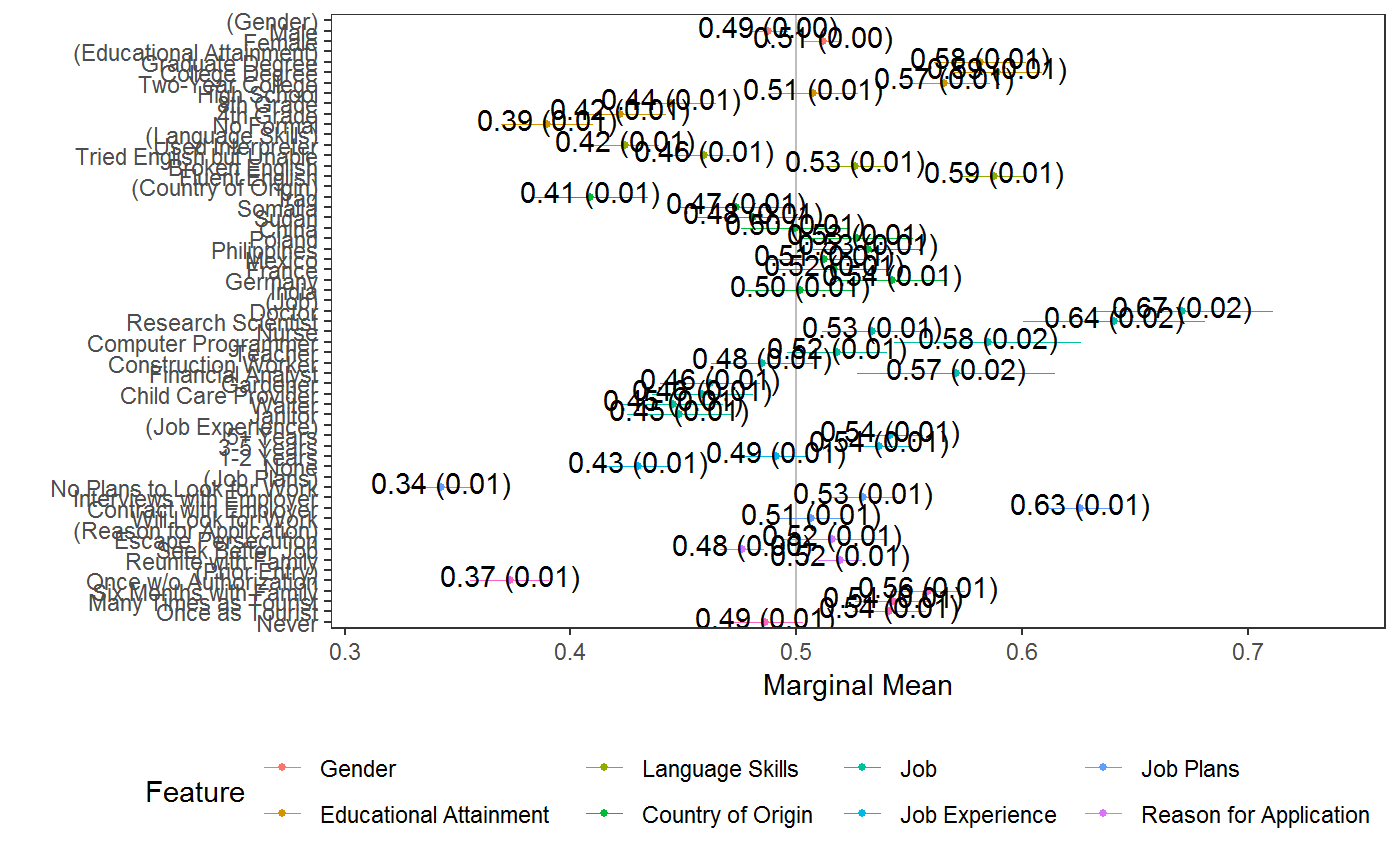
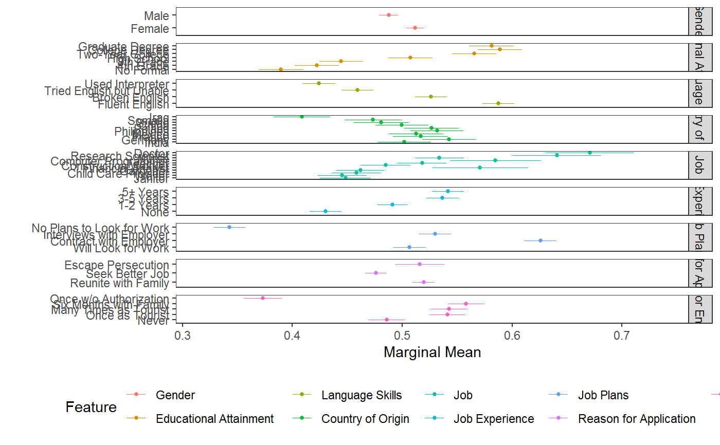
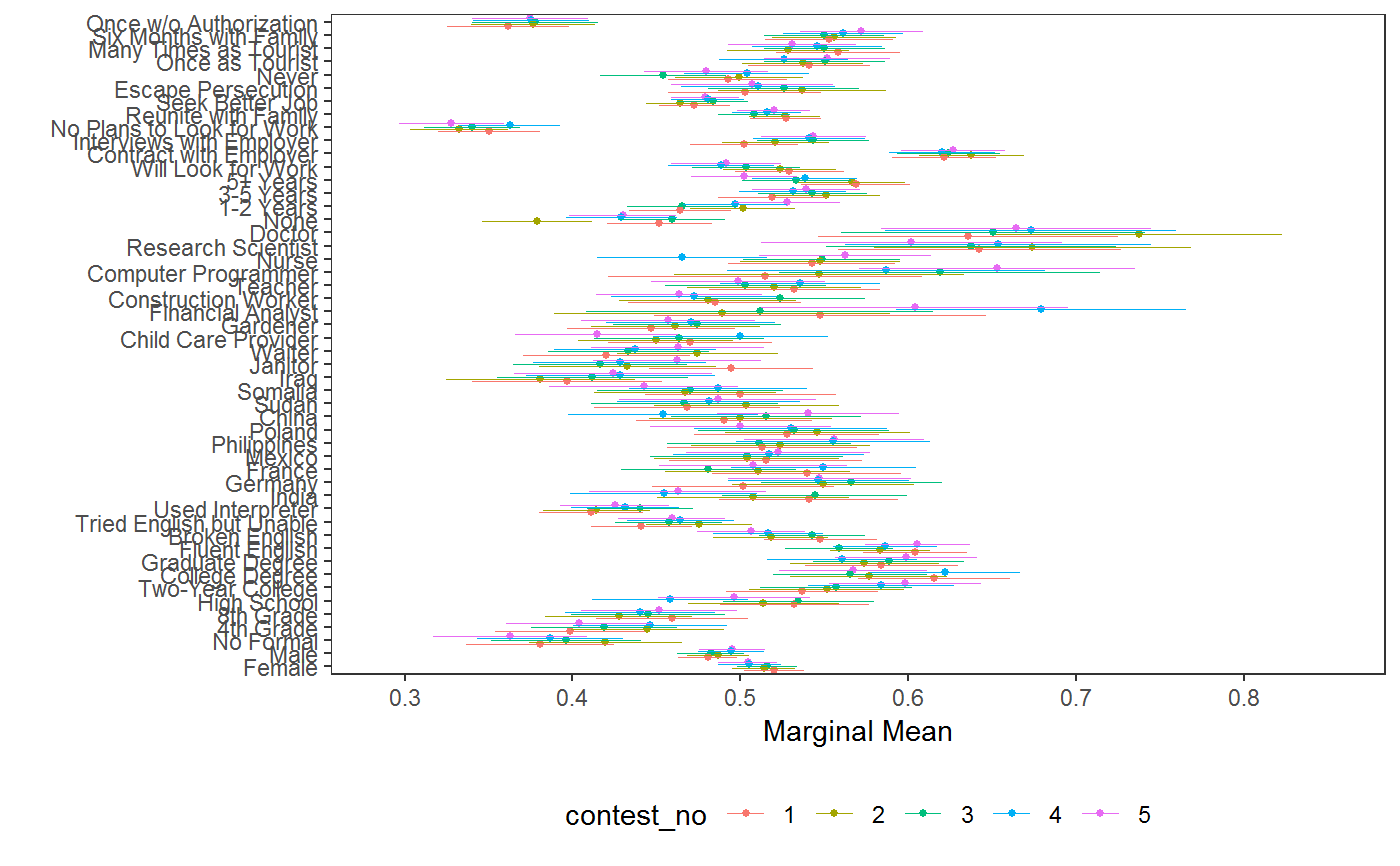
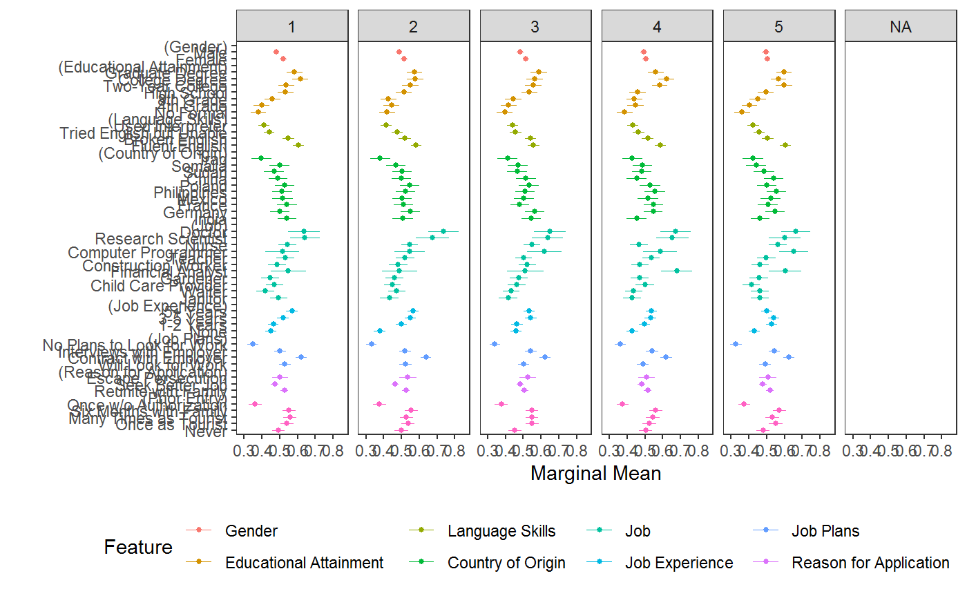
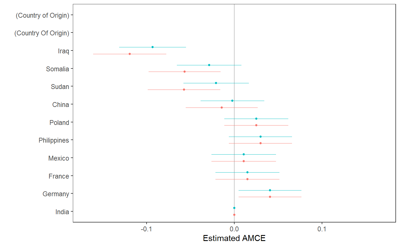
# load data
data("immigration")
immigration$contest_no <- factor(immigration$contest_no)

# calculate MMs
d1 <- mm(immigration, ChosenImmigrant ~ Gender + Education +
         LanguageSkills + CountryOfOrigin + Job + JobExperience +
         JobPlans + ReasonForApplication + PriorEntry, id = ~ CaseID)

# plot MMs
## simple plot
(p <- plot(d1, vline = 0.5))

## gridlines to aid interpretation
p + ggplot2::theme_grey()

## monochrome bars
p + scale_color_manual(values = rep("black", 9))
#> Scale for 'colour' is already present. Adding another scale for 'colour',
#> which will replace the existing scale.

## plot with estimates shown as text labels
p + ggplot2::geom_text(
  aes(label = sprintf("%0.2f (%0.2f)", estimate, std.error)),
  colour = "black", position = position_nudge(y = .5)
)
#> Warning: Removed 9 rows containing missing values (geom_text).

## plot with facetting by feature
plot(d1, feature_headers = FALSE) +
  ggplot2::facet_wrap(~feature, ncol = 1L,
                      scales = "free_y", strip.position = "right")

# MMs split by profile number
stacked <- cj(immigration, ChosenImmigrant ~ Gender +
              Education + LanguageSkills + CountryOfOrigin + Job + JobExperience +
              JobPlans + ReasonForApplication + PriorEntry, id = ~ CaseID,
              estimate = "mm", by = ~ contest_no)

## plot with grouping
plot(stacked, group = "contest_no", feature_headers = FALSE)

## plot with facetting
plot(stacked) + ggplot2::facet_wrap(~contest_no, nrow = 1L)

## plot with shapes instead of colors for groups
plot(stacked, group = "contest_no", vline = 0.5) +
 aes(shape = contest_no) + # map group to `shape` aesthetic
 scale_shape_manual(values=c(1, 2, 3, 4, 5)) +
 scale_discrete_manual(values=rep("black", 5)) # optionally, override colour
#> Error in manual_scale(aesthetics, values, ...): argument "aesthetics" is missing, with no default

# estimate AMCEs over different subsets of data
reasons12 <- subset(
  immigration, ReasonForApplication %in% levels(ReasonForApplication)[1:2]
)
d2_1 <- cj(immigration, ChosenImmigrant ~ CountryOfOrigin, id = ~ CaseID)
d2_2 <- cj(reasons12, ChosenImmigrant ~ CountryOfOrigin, id = ~ CaseID,
           feature_labels = list(CountryOfOrigin = "Country Of Origin"))
d2_1$reasons <- "1,2,3"
d2_2$reasons <- "1,2"
plot(rbind(d2_1, d2_2), group = "reasons")
# }