Conjoint feature frequencies

Tabulate and visualize conjoint features, and their display frequencies and proportions

cj_freqs(
  data,
  formula,
  id = NULL,
  weights = NULL,
  feature_order = NULL,
  feature_labels = NULL,
  level_order = c("ascending", "descending"),
  ...
)

cj_props(data, formula, id, weights = NULL, margin = NULL, ...)

cj_table(
  data,
  formula,
  feature_order = NULL,
  feature_labels = NULL,
  level_order = c("ascending", "descending"),
  include_reference = FALSE,
  ...
)

Arguments

data	A data frame containing variables specified in formula. All RHS variables should be factors; all levels across features should be unique.
formula	An RHS formula specifying conjoint features to tabulate. All RHS variables should be factors; all levels across features should be unique.
id	An RHS formula specifying a variable holding respondent identifiers, to be used for clustering standard errors. By default, data are unclustered.
weights	An (optional) RHS formula specifying a variable holding survey weights.
feature_order	An (optional) character vector specifying the names of feature (RHS) variables in the order they should be encoded in the resulting data frame.
feature_labels	A named list of “fancy” feature labels to be used in output. By default, the function looks for a “label” attribute on each variable in formula and uses that for pretty printing. This argument overrides those attributes or otherwise provides fancy labels for this purpose. This should be a list with names equal to variables on the righthand side of formula and character string values; arguments passed here override variable attributes.
level_order	A character string specifying levels (within each feature) should be ordered increasing or decreasing in the final output. This is mostly only consequential for plotting via plot.cj_mm, etc.
...	Ignored.
margin	A numeric value passed to prop.table. If NULL overall proportions are calculated.
include_reference	A logical indicating whether to include a “reference” column that indicates whether a feature level is the reference category for that feature. Default is FALSE.

Value

A data frame of class “cj_freqs”, “cj_props”, etc.

Details

These functions provide related but slightly different functionality. cj_table simply creates a data frame of features and their levels, which is useful for printing. cj_props provides tidy proportion tables to examine cross-feature restrictions in conjoint designs that are not equally randomized. This enables, for example, tabulation and visualization of complete restrictions (where combinations of two or more features are not permitted), as well as calculation of AMCEs for constrained designs appropriately weighted by the display proportions for particular combinations of features.

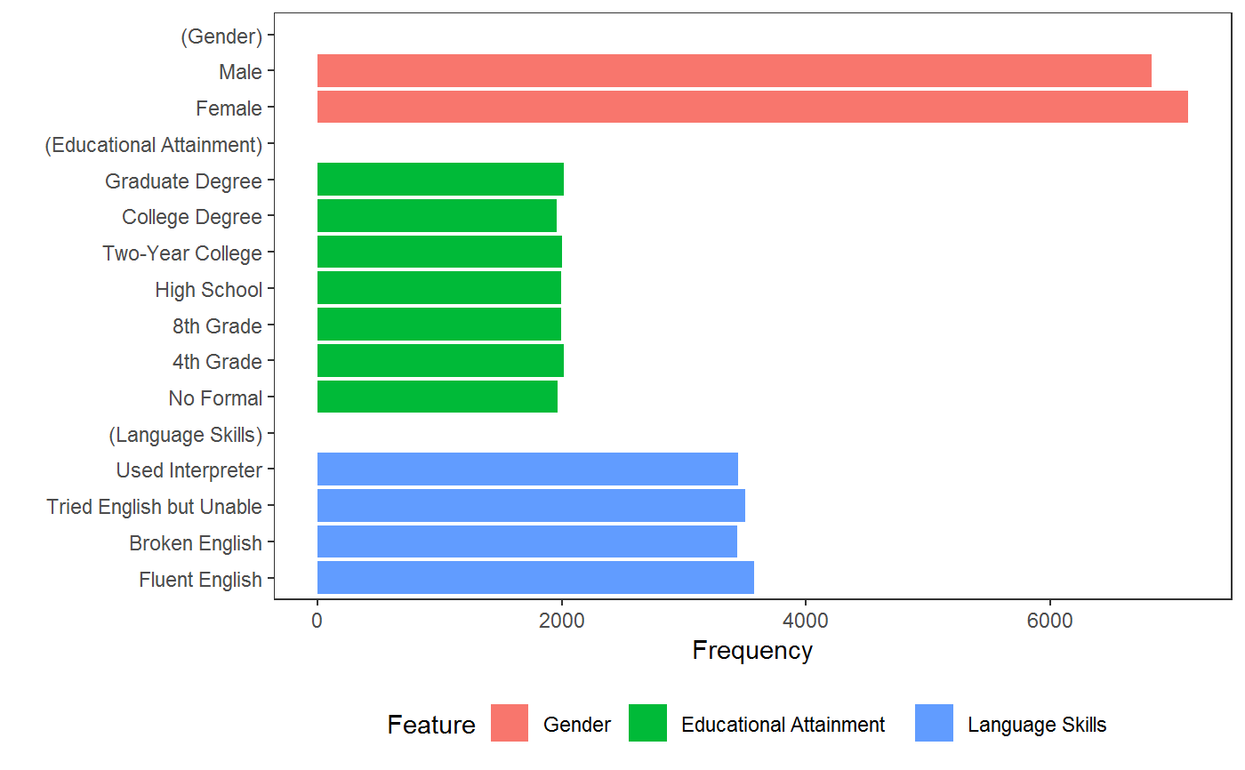
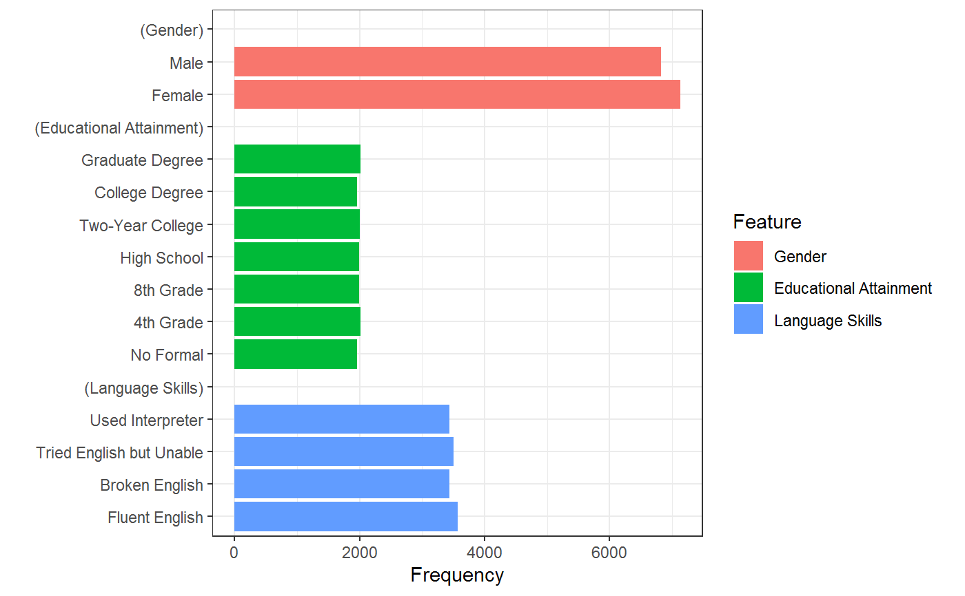
cj_freqs provides marginal display frequencies, which are a descriptive check on the presentation of individual conjoint features (for example, to ensure equal or intentionally unequal appearance of levels). This is mostly useful for plotting functionality provided in plot.cj_freqs, which provides barcharts for the frequency with which each level of each feature was presented.

See also

plot.cj_mm

Examples

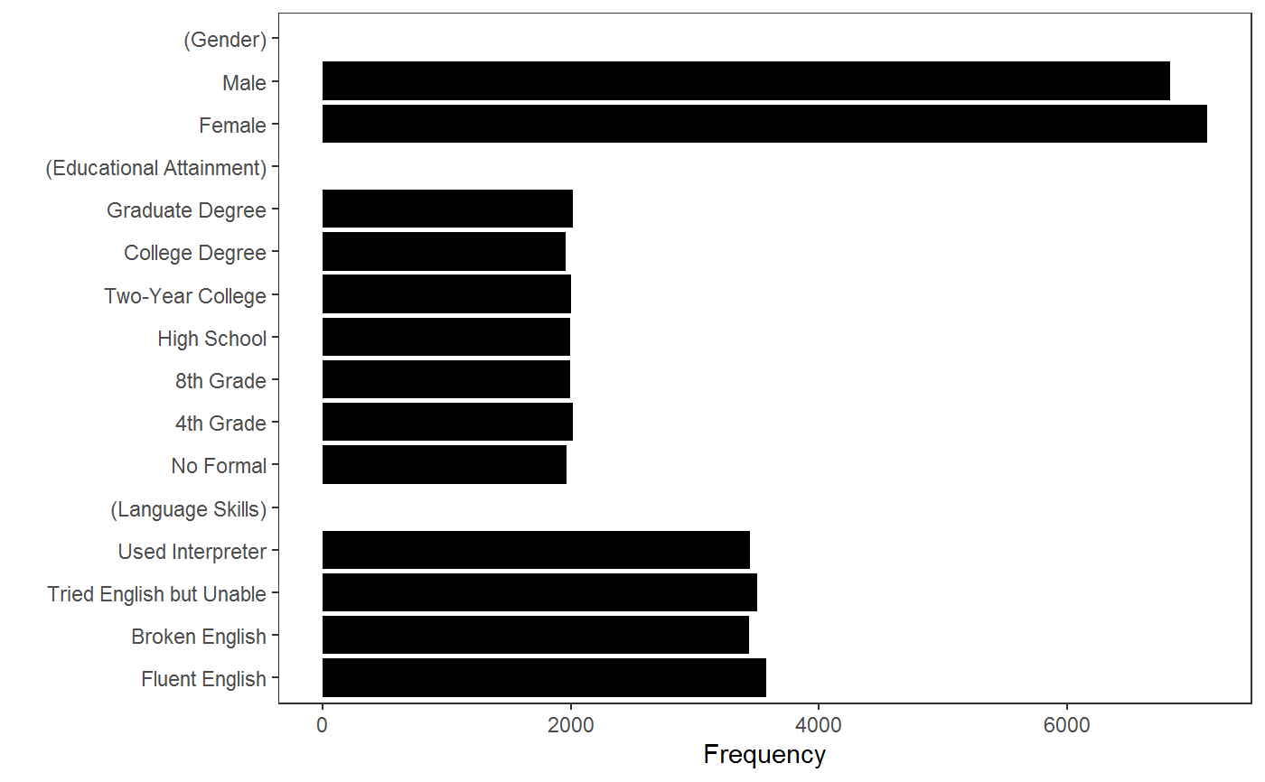
data(immigration)
# identify all levels
cj_table(immigration, ~ Gender + Education + LanguageSkills)
#>                   feature                    level
#> 1                  Gender                   Female
#> 2                  Gender                     Male
#> 3  Educational Attainment                No Formal
#> 4  Educational Attainment                4th Grade
#> 5  Educational Attainment                8th Grade
#> 6  Educational Attainment              High School
#> 7  Educational Attainment         Two-Year College
#> 8  Educational Attainment           College Degree
#> 9  Educational Attainment          Graduate Degree
#> 10        Language Skills           Fluent English
#> 11        Language Skills           Broken English
#> 12        Language Skills Tried English but Unable
#> 13        Language Skills         Used Interpreter
cj_table(immigration, ~ Gender + Education + LanguageSkills, include_ref = TRUE)
#>                   feature                    level reference
#> 1                  Gender                   Female      TRUE
#> 2                  Gender                     Male     FALSE
#> 3  Educational Attainment                No Formal      TRUE
#> 4  Educational Attainment                4th Grade     FALSE
#> 5  Educational Attainment                8th Grade     FALSE
#> 6  Educational Attainment              High School     FALSE
#> 7  Educational Attainment         Two-Year College     FALSE
#> 8  Educational Attainment           College Degree     FALSE
#> 9  Educational Attainment          Graduate Degree     FALSE
#> 10        Language Skills           Fluent English      TRUE
#> 11        Language Skills           Broken English     FALSE
#> 12        Language Skills Tried English but Unable     FALSE
#> 13        Language Skills         Used Interpreter     FALSE

# display frequencies
(f <- cj_freqs(immigration, ~ Gender + Education + LanguageSkills, id = ~ CaseID))
#>      statistic                feature                    level estimate
#> 1  frequencies                 Gender                   Female     7130
#> 2  frequencies                 Gender                     Male     6830
#> 3  frequencies Educational Attainment                No Formal     1964
#> 4  frequencies Educational Attainment                4th Grade     2018
#> 5  frequencies Educational Attainment                8th Grade     1998
#> 6  frequencies Educational Attainment              High School     1994
#> 7  frequencies Educational Attainment         Two-Year College     2005
#> 8  frequencies Educational Attainment           College Degree     1963
#> 9  frequencies Educational Attainment          Graduate Degree     2018
#> 10 frequencies        Language Skills           Fluent English     3576
#> 11 frequencies        Language Skills           Broken English     3440
#> 12 frequencies        Language Skills Tried English but Unable     3501
#> 13 frequencies        Language Skills         Used Interpreter     3443

# restrictions
## check display proportions
cj_props(immigration, ~ Job, id = ~ CaseID)
#>                    Job Proportion
#> 1              Janitor 0.11697708
#> 2               Waiter 0.12335244
#> 3  Child Care Provider 0.12578797
#> 4             Gardener 0.11833811
#> 5    Financial Analyst 0.03488539
#> 6  Construction Worker 0.11876791
#> 7              Teacher 0.12098854
#> 8  Computer Programmer 0.03882521
#> 9                Nurse 0.12399713
#> 10  Research Scientist 0.03868195
#> 11              Doctor 0.03939828
## check which combinations were not allowed
subset(cj_props(immigration, ~ Job + Education, id = ~ CaseID), Proportion == 0)
#>                    Job   Education Proportion
#> 5    Financial Analyst   No Formal          0
#> 8  Computer Programmer   No Formal          0
#> 10  Research Scientist   No Formal          0
#> 11              Doctor   No Formal          0
#> 16   Financial Analyst   4th Grade          0
#> 19 Computer Programmer   4th Grade          0
#> 21  Research Scientist   4th Grade          0
#> 22              Doctor   4th Grade          0
#> 27   Financial Analyst   8th Grade          0
#> 30 Computer Programmer   8th Grade          0
#> 32  Research Scientist   8th Grade          0
#> 33              Doctor   8th Grade          0
#> 38   Financial Analyst High School          0
#> 41 Computer Programmer High School          0
#> 43  Research Scientist High School          0
#> 44              Doctor High School          0

# \donttest{
# plotting
(p <- plot(f))
#> Warning: Removed 3 rows containing missing values (position_stack).

## change ggplot2 theme
p + ggplot2::theme_bw()
#> Warning: Removed 3 rows containing missing values (position_stack).

## monochrome bars
p + ggplot2::scale_fill_manual(values = rep("black", 9)) +
  ggplot2::theme(legend.position = "none")
#> Scale for 'fill' is already present. Adding another scale for 'fill', which
#> will replace the existing scale.
#> Warning: Removed 3 rows containing missing values (position_stack).
# }